Linear regression is a linear approach ( we use a linear function) for modelling the relationship between two continuous variables, a dependent and an independent variable. The linear model allows us to find the value of an dependent variable when we know the independent value. We only have to feed the value to our model.

Example, let's say we have a linear function: y = ax + b x = independent variable (weight) y = dependent variable (height) a = slope of the line of a function b = y intercept or bias

We can predict the height using weight by putting in the value of weight x in the function.

In this post, we will try to implement a simple linear regression model using deep learning framework PyTorch.

Contents:

• Basic linear model and prediction
• Initializing linear class
• Custom modules
• Training a linear model using data set

Basic linear model and prediction

Create a simple linear model and predict the values. We will use the following function:

• y = w*x + b, equation of line w=weight or slope, b=bias or y intercept

First, install torch if it is not already installed in the system:

$ pip install torch

Using simple linear model for prediction:

import torch

w = torch.tensor(3.0, requires_grad=True)   # give a random value of value 3
b = torch.tensor(1.0, requires_grad=True)

# define the forward function
def forward(x):
    y = w*x + b 
    return y

x = torch.tensor(2) 
forward(x)   # we can predict as many input as we want, say forward([[4], [7]])but

Initializing linear class

import torch
from torch.nn import Linear

torch.manual_seed(1)    # sets a seed for generating random values, when creating a linear model it will be given a random values for the linear class and to ensure random values are assigned to weight and bias, seed can be any number
model = Linear(in_features=1, out_features=1)    # create a linear model, which means for every one prediction i.e for every output, there is one in_feature, single input
print(model.bias, model.weight)    # To determine model's parameters

x = torch.tensor([2.0])
print(model(x))   # prediction using model

x = torch.tensor([[2.0], [3.3]])
print(model(x))  # prediction for multiple inputs

Custom modules

A robust and efficient way of building neural networks with PyTorch. We will build our own simple linear model using custom modules.

import torch
import torch.nn as nn

class LR(nn.Module):   # Creating new class for Linear regression. Inherit from base class Module
    def __init__(self, input_size, output_size):   # Use this constructor to initialize new instances of new class
        super().__init__()   # call super method for inheritance 
        self.linear = nn.Linear(input_size, output_size)   # initialize the instances

  # create a forward method so that it can be accessed using model object to predict
    def forward(self, x):
        pred = self.linear(x)
        return pred

torch.manual_seed(1)
# initialize new model and its instances
model = LR(1, 1)
# print(list(model.parameters()))   # print it in the form of list for better viewing

x = torch.tensor([1.0])
print(model.forward(x))   # call the method forward to predict 

x = torch.tensor([[1.0], [2.0]])   # two predictions based on two independent variables
print(model.forward(x))

Training linear model class

First we will create data set. After that we will train the model to develop new weight and bias values based on previously labeled data rather than working with random parameters.

import torch
import torch.nn as nn
import matplotlib.pyplot as plt
import numpy as np



# creating datasets
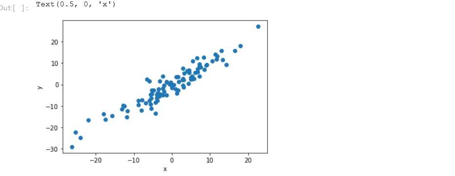
X = torch.randn(100, 1)*10 # shape of tensor to be 100 rows and 1 col, returns tensor filled with random numbers which are normally distributed
y = X + 3*torch.randn(100, 1) # add a noise to y data so that the data points to be relatively spaced out around 0, small standard deviation, 
# print(X) # normally distributed tensors, relatively small numbers centered around 0 so we multiply by 10 to set larger range
plt.plot(X.numpy(), y.numpy(), 'o')  #'y gives a straight dotted line if y = X which shows al data points are normally distributed within X
plt.ylabel('y')
plt.xlabel('x')

# now that we have created a noisy dataset, it is time to train our model

class LR(nn.Module):  # Creating new class for Linear regression. Inherit from base class Module
    def __init__(self, input_size, output_size):  # Use this constructor to initialize new instances of new class
        super().__init__()  # call super method for inheritance 
        self.linear = nn.Linear(input_size, output_size)  # initialize the instances

   # create a forward method so that it can be accessed using model object to predict
    def forward(self, x):
        pred = self.linear(x)
        return pred

torch.manual_seed(1)
# initialize new model and its instances
model = LR(1, 1)
# print(list(model.parameters()))  # print it in the form of list for better viewing

# Obtain model parameters by unpacking the model 
[w, b] = model.parameters()
# print(w, b)   # we see that weight is a 2 dimensional array with one row and one column
# w1 = w[0][0].item()   # access using row 0 and col 0 index for weight and apply .item() method to print single python number from both tensor values
# b1 = b[0].item()  # single item at 0th index
# print(w1, b1)   # print parameters

# for clean method create a function to get the parameters
def get_params():
    return(w[0][0].item(), b[0].item())

# plot the linear model along side the data points
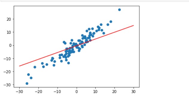
def plot_fit(title):
    plt.title = title

    # To determine neumerical expressions for x1 and y1
    w1, b1 = get_params()  
    x1 = np.array([-30, 30])   # x values between -30 to 30, make it an array not tensor to   make it compatible with pyplot
    y1 = w1 * x1 + b1   # From the two x points from -30 to 30 we can get two y points
    plt.plot(x1, y1, 'r')   # plot it as redline
    plt.scatter(X, y)   # plot datasets
    plt.show()

plot_fit('Initial Model')   # call the plot. Since it is not the plot we want, we will need to use gradient descent to update its parameters

Loss Function

We will now find the parameters of a line that fits the data well

• (y - y_hat)**2

• (y - wx + b)**2

• (y - wx + 0)**2 # keep the bias to 0 by removing bias

• (y - wx)**2

loss = (3 - w(-3))**2 for (-3, 3), the

• value of w = -1 gives the minimum error = 0

Gradient descent

Gradient descent is an optimizing algorithm which will try to minimize the error function of a linear model until it is trained to fit into our data. It is important to use gradient descent in creating a linear model because it will try to update the position of a line to best fit into the data set.

How do we train our model to determine the weight parameters which will minimize the error function ( can be done with gradient descent).

First we compute the derivative of the loss function.

• loss = (3 - w(-3))**2
• f'(w) = 18(w+1)

Then, subtract in the current weight value of the line. Whatever the weight may be, this will give the gradient value(f'(w)).

• w1 = w0 - f'(w)

The gradient value is subtracted from the current weight w0 to give the new updated weight, w1. The new weight should result in a smaller error than the previous one. We keep doing that iteratively until we obtain a small error, until we obtain the optimal parameters for our linear model to fit the data.

We are descending with the gradient. To ensure optimal result, one should descend with really small steps and we do this by multiplying a gradient with a learning rate, small number.

• w1 = w0 - learning_rate*f'(w)

Mean Squared Error

Similar to error function but here now we consider the biases

• (y - wx + b) ** 2

• MSE = 1/N sum(y ith - mean(y ith))*2

• f(m, b) = 1/N sum(y ith- (mx ith+ b))*2

New weight

• m1 = m0 - learningrate * f'(m)

new bias

• b1 = b0 - learnigrate * f'(b)

Training - Code Implementation

# builtin loss function
criterion = nn.MSELoss()
# optimizer, stochastic gradient descent 
optimizer = torch.optim.SGD(model.parameters(), lr=0.01)  # stochastic gradient descent minimizes total loss one sample at a time

# training our model
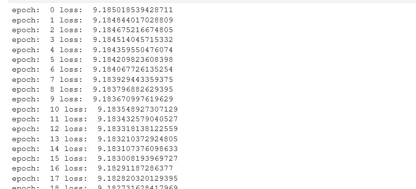
epochs = 100 # iterative process,  when we iterate once over the entire datset, we calculate the error function and back prapagate the gradient of error function to update the weights
losses = []
for i in range(epochs):
    y_pred = model.forward(X)
    loss = criterion(y_pred, y)
    print("epoch: ", i, "loss: ", loss.item())

    losses.append(loss) # accumulate loss in the losses list
    # set gradients to zero
    optimizer.zero_grad()

    # minimize the loss at every epoch for the gradients calculated using the derivative
    loss.backward()
    optimizer.step() # update the model parameters

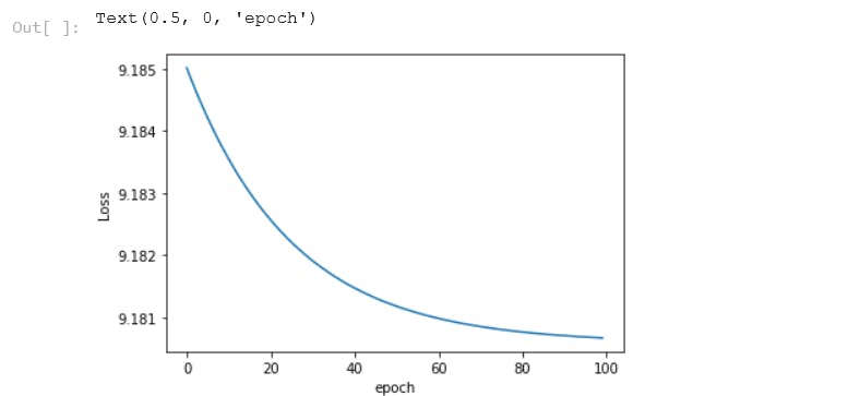
# plot the loss on graph
plt.plot(range(epochs), losses)
plt.ylabel('Loss')
plt.xlabel('epoch')

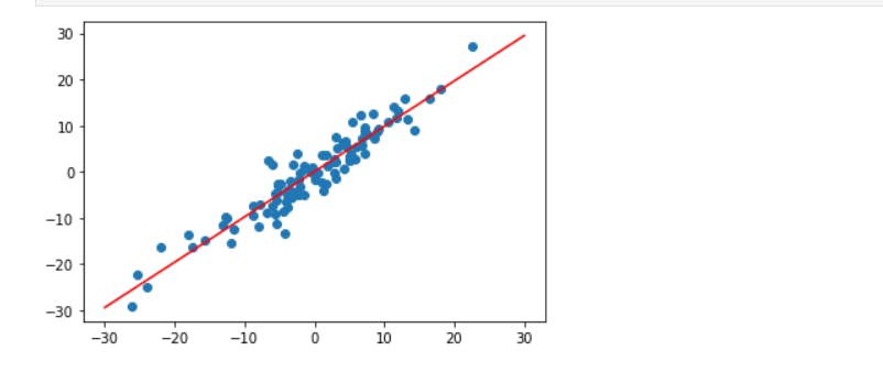
plot_fit('Trained Model') # calling trained fit model

Reference: Video